Communication in OPENATOM

The ten phases described in the previous section are parallelized by decomposing the physical system into 15 chare arrays of different dimensions (ranging between one and four). A description of these objects and communication between them follows:

1. GSpace and RealSpace: These represent the g-space and real-space representations of the electronic states. They are 2-dimensional arrays with states in one dimension and planes in the other. They are represented by $G(s, p) [n_s \times N_g]$ and $R(s, p) [n_s \times N]$ respectively. GSpace and RealSpace interact through transpose operations in Phase I and hence all planes of one state of GSpace interact with all planes of the same state of RealSpace. RealSpace also interacts with RhoR through reductions in Phase II.

2. RhoG and RhoR: They are the g-space and real-space representations of electron density and are 1-dimensional (1D) and 2-dimensional (2D) arrays respectively. They are represented as $G_{\rho}(p) [N_{g \rho}]$ and $R_{\rho}(p, p') [(N / N_y) \times N_y]$. RhoG is obtained from RhoR in Phase III through two transposes.

3. RhoGHart and RhoRHart: RhoR and RhoG are used to compute their Hartree and exchange energy counterparts through several 3D FFTs (in Phase IV). This involves transposes and point-to-point communication. RhoGHart and RhoRHart are 2D and 3D arrays represented by $G_{HE}(p, a) [N_{gHE} \times n_{atom-type}]$ and $R_{HE}(p, p',$ $a) [(1.4N / N_y) \times N_y \times n_{atom-type}]$.

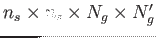
4. Particle and RealParticle: These two 2D arrays are the g-space and real-space representations of the non-local work and denoted as $G_{nl}(s, p)\ [n_s \times N_g]$ and $R_{nl}(s, p) [n_s \times 0.7N]$. Phase X for the non-local computation can be overlapped with Phases II-VI and involves communication for two 3D FFTs.

5. Ortho and CLA_Matrix: The 2D ortho array, $O(s, s')$ does the post-processing of the overlap matrices to obtain the T-matrix from the S-matrix. There are three 2D CLA_Matrix instances used in each of the steps of the inverse square method (for matrix multiplications) used during orthonormalization. In the process, these arrays communicate with the paircalculator chare arrays mentioned next.

6. PairCalculators: These 4-dimensional (4D) arrays are used in the force regularization and orthonormalization phases (VII and VIII). They communicate with the GSpace, CLA_Matrix and Ortho arrays through multicasts and reductions. They are represented as 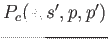$P_c(s, s', p, p')$ of dimensions $n_s \times n_s \times N_g \times N_{g}'$. A particular state of the GSpace array interacts with all elements of the paircalculator array which have this state in one of its first two dimensions.

7. Structure Factor: This is a 3D array used when we do not use the EES method for the non-local computation.